How to Use Indexed Universal Life (IUL) to Increase Portfolio Returns

Rajiv Rebello
Author
February 19, 2022

Author

An alternative to investing in short-term or long-term bonds is to invest in the equity markets with a floor and a cap through indexed universal life (IUL) policies. This can provide higher returns than investing in whole life insurance or investing in bonds directly. In exchange for these higher expected returns, investors are taking on more investment and insurance risk than investing in bonds—but less investment risk than investing in the equity markets directly. So there’s a great risk-adjusted opportunity here.
Since a floored and capped strategy essentially caps the upside potential, an IUL strategy will almost never outperform a traditional equity strategy over the long-term. However, in the event of an equity market crash, an IUL will also not absorb heavy losses while a pure equity strategy will.
Therefore, the idea behind using IULs as part of a long-term financial planning/investment structuring strategy is not to take assets out of an equity strategy to invest in IULs since doing so will hurt long-term portfolio returns. Rather, the goal is to take the part of the portfolio that would have been allocated to short-term or long-term bonds and invest that portion in an IUL strategy. Doing so will provide higher gross returns and higher after-tax returns over the long-term than investing in short-term or long-term bonds directly and less volatility than increasing a portfolios allocation to equity investments in the wake of low bond yields and rising interest rates.
Increasing after-tax returns without increasing volatility by investing in IUL policies
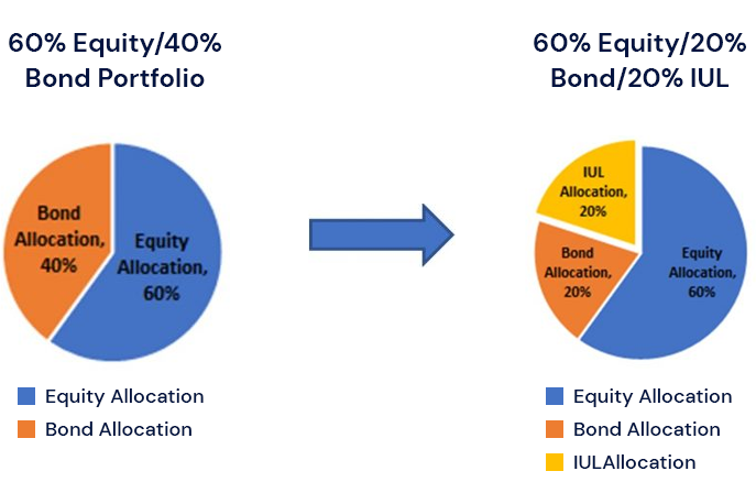
In a low bond yield and increasing interest rate environment, financial advisors can provide higher risk-adjusted returns in their portfolio construction by taking assets out of the bond portfolio and allocating it to an IUL policy. Doing so allows higher after-tax risk adjusted returns without exposing clients to the full volatility of the equity markets.
Sample equity indexed returns vs equity capped and floored returns
| Year | Sample Equity Index Return | Equity Index Return Capped at 8% and Floored at 0% |
|---|---|---|
| 1 | 20% | 8% |
| 2 | 13% | 8% |
| 3 | -23% | 0% |
| 4 | 4% | 4% |
| 5 | 15% | 8% |
The table shows sample equity returns relative to the returns that would be earned if the equity index was capped at 8% and floored at 0%.
Over the long-term the underlying equity index will always outperform the capped and floored equity strategy since the underlying index will have more upside gain. But the capped and floored equity strategy will also have significantly less volatility in its returns since it limits the downside risk.
By capping the upside return and flooring the downside return, a floored and capped strategy can provide access to the equity markets without the full volatility of equity investments.
In a low yield and rising interest rate environment, investing in such a strategy can be a great alternative to investing in bonds—particularly on an after-tax basis. The reason for this is that bonds are low yielding and taxed at high ordinary income rates. Furthermore, in a rising interest rate environment bond investments will take a large upfront loss. So by taking a portion of a client’s portfolio that would otherwise be allocated to bonds and investing in a capped and floored equity strategy instead, clients can achieve higher risk-adjusted returns on an after-tax basis.
Clients can achieve this capped and floored equity strategy themselves by buying and selling options on the desired equity index. But this requires some level of sophistication on behalf of the investor as well as the ability to buy options at cost effective prices. On the other hand, index universal life (IUL) is a life insurance policy that allows for investors to get access to this same equity floored and capped strategy while leveraging the insurance company’s ability to buy options at wholesale prices with their large balance sheet. In exchange for providing access to this strategy, the insurance company charges clients insurance expenses. While these expenses do eat into the returns, the insurance company also makes the returns tax-free to clients. So as long as the gross returns and tax-savings are larger than the insurance expenses, then the client can achieve significant benefit from utilizing the IUL strategy in place of low-yielding bonds.
In order to determine the investing and tax-benefits of an IUL strategy relative to investing in bonds directly, we can stochastically simulate equity returns, bond returns, and a capped/floored equity strategy to see exactly what the “tax-alpha” would be by implementing an IUL strategy over a bond strategy.
As the table below shows, an IUL strategy can provide higher after-tax returns than a taxable bond strategy while also providing lower volatility than investing directly in equities.
After-tax returns of IUL vs Equity and Bond strategies
| Asset Strategy | After-tax 30 year mean return | Standard Error | Sharpe Ratio in comparison to Bond Strategy | Sortino Ratio in comparison to 1.37% after-tax yield |
|---|---|---|---|---|
| Equity | 6.98% | 2.41% | 2.33 | 3.29 |
| IUL | 3.42% | 0.80% | 2.55 | 3.44 |
| Bond | 1.58% | 0.32% | 0.66 | 0.88 |
As the table above shows, on an after-tax basis the IUL strategy has lower returns than the pure equity investment strategy—but it also has lower volatility than that of the equity strategy.
In comparison to the bond strategy, the IUL strategy has significantly higher returns with only a small increase in volatility. Therefore on a risk-adjusted basis, the IUL strategy can provide significant value over direct bond investing as the Sharpe Ratio comparison identifies.
Simulation assumptions:
The above table shows that the IUL strategy provides significantly greater after-tax returns than the bond strategy with only a small increase in volatility. As measured by the calculated Sharpe ratio, the IUL strategy actually provides higher after-tax adjusted returns than even the pure equity strategy. In fact, the IUL provides such immense value over bonds in a low-yield environment that the insurance expenses can be almost tripled before the bond strategy starts to become a better option as indicated in the table below.
IUL After-Tax Returns with Varying Expense Ratios in Comparison to After-Tax
| Asset Strategy | Mean after-tax 30 year return | Standard Error | Sharpe Ratio in comparison to Bond Strategy | Sortino Ratio in comparison to 1.37% after-tax yield |
|---|---|---|---|---|
| IUL with 0% of IUL expenses | 4.86% | 0.84% | 4.08 | 5.51 |
| IUL with 100% of IUL expenses | 3.42% | 0.32% | 2.55 | 3.44 |
| IUL with 200% of IUL expenses | 2.34% | 0.55% | 1.28 | 2.75 |
| IUL with 285% of IUL expenses | 1.58% | 0.75% | 0.28 | 0.37 |
| Bond | 1.58% | 0.32% | 0.66 | 0.88 |
Expenses in a decent IUL policy often take up to 1.25%-2% of the return of the policy. It would take an expense ratio of 258% of the normal IUL expense for the IUL policy to start underperforming the bond strategy in this low yield environment.
Simulation assumptions:
IUL policies often get a bad wrap when actual returns on the policy don’t line up with what the policyowner expected to get prior to investing in the policy. Part of the blame for this is due to insurance companies providing misleading illustrations and bonus credits which can hide high back-end expenses. However, part of poor performance in IUL policies is also due to poor policyowner behavior by clients who don’t understand the complexity of the policies they acquired or how to manage the investment and insurance risk.
When utilizing an IUL policy as part of a tax-efficient financial planning strategy, clients and their advisors need to be aware of the following:
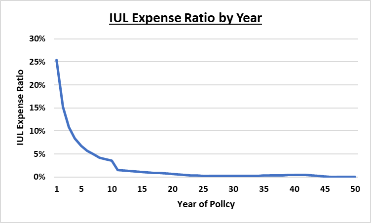
Most investors are used to seeing a level expense charge every year of their investment (like a 1% yearly management fee or advisory fee charge every year). Life insurance expense ratios don’t work like that. Life insurance expense ratios are typically extremely high in the early years and extremely low in the later years (if the policy has been funded well) as illustrated in the chart below.
The high early year expenses mean that the early year returns of an IUL policy will be low in comparison to a bond strategy. However, the low expenses in the later years of the policy–in combination with the tax-free growth—results in the IUL policy far exceeding the growth of the bond strategy as illustrated in the graph below.
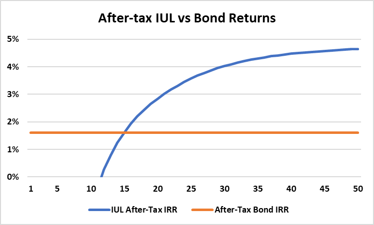
While high early year expenses initially eat up the benefits of the IUL policy, the low expenses and tax-free growth of the IUL policy in the later years far exceed that of the bond strategy. The longer the policyowner keeps the policy, the higher their IRR due to the lower expenses in the later years.
Assumptions:
Bond return: 3.5%
Ordinary Income Tax Rate: 54.2%
For those looking to maximize the value of the IUL policy they need to ensure that they both utilize a low-expense product and intend on keeping it for the long-term.
IUL policies are able to protect investor downside by purchasing put options on that index. To help pay for these options, insurance companies sell call options that cap the upside the policyowner can receive. The price of these options is dependent on how volatile the underlying index is. The more volatile the index, the more expensive the price of the put options, and the lower the cap is for the policyowner.
Since 1 year options are more volatile/expensive than multi-year options, policyowners can receive higher returns from an IUL policy that credits interest every few years instead of every year. The downside is that the policyowner will have to wait a few years to see the interest credited to their policy. However, since this is a long-term investment/retirement vehicle anyways, the extra delay in waiting for the interest to be credited shouldn’t be a hindrance. At any rate, the extra 100 basis points in expected return—which is approximately a 20%-25% increase over the annual point-to-point strategy—should make this minor inconvenience more than worth it.
2 year point-to-point strategy vs 1 year point-point strategy
| IUL Strategy | 20 Year Mean IRR | 30 Year Mean IRR | 40 Year Mean IRR | 50 Year Mean IRR |
|---|---|---|---|---|
| IUL with 1-year point-to-point strategy | 2.39% | 3.42% | 3.81% | 4.08% |
| IUL with 2-year point-to-point strategy | 3.32% | 4.37% | 4.77% | 4.99% |
Choosing a 2-year crediting strategy can increase the expected IRR by nearly 100 basis points which is 20%-25% higher than the 1 year point-to-point crediting strategy
Simulation Assumptions:
1-Year Point-to-Point: 8% mean return, 15% standard deviation, 8% cap
2-Year Point-to-Point: 8% mean return, 15% standard deviation, no cap, 84% participation rate, 3% spread
Insurance agents tend to show illustrations to potential clients that highlight the benefits of the policy while hiding the downside. Cost of insurance rates can be high in the later years of a policy. However, the effect of these can be minimized if the policy has been well funded and the underlying investment strategy has performed well. However, if the opposite is true and the policy has been improperly funded or the index returns are poor, then insurance expenses in the later years can eat up a lot of the investment return.
This is why simply showing a high level crediting rate—particularly if the crediting rate is unrealistic—can hide the insurance and investment expense in the later years.
In order to truly get an accurate understanding of the risk of the policy, clients need to illustrate the effects of the policy under two different crediting rates: one that is lower than expected, and one that is higher than expected. The client can then roughly see how sensitive the policy’s returns are to changes in the investment rate. The client can then use this same sensitivity test to compare the results of one carrier against another.
Sensitivity Testing IUL returns by lowering the crediting rate
| A | B | C = (B-A)/A | |
| Product | 40 year IRR at 6% crediting rate | 40 year IRR at 4% crediting rate | % loss due to crediting rate reduction |
|---|---|---|---|
| IUL Product A | 5.35% | 3.26% | -39.07% |
| IUL Product B | 5.20% | 3.65% | -29.81% |
In the table above, Product A outperforms Product B at a 6% crediting rate but underperforms Product B at a 4% crediting rate. This implies that Product A has higher expenses in the product that can be hidden by using a higher illustrated crediting rate. Sensitivity testing products by lowering the crediting rate assumption can help reveal the effects of these hidden expenses.
Some insurance carriers often offer “bonus crediting rates” as a benefit to get clients to choose their insurance company over others. Sometimes this “bonus crediting rate” is offered for “free” (i.e. they are not charging for it directly, but are indirectly increasing other expenses in the policy to cover it) and sometimes it’s offered at an explicit charge.
To keep things simple, let’s assume that the carrier is offering a 20% bonus interest crediting rate in exchange for an explicit 1% charge on the policy’s account value. What crediting rate makes this charge viable? Well, we can do some quick math here and figure it out. As long as the crediting rate is 5% or greater, then the bonus crediting rate is always worth the explicit charge (20% of 5% is 1%, so the 1% bonus crediting rate is equal to the 1% charge).
As long as an agent illustrates this policy with a level crediting rate of 5% or higher, then it will appear that the policyowner always comes up ahead since the bonus crediting rate is always equal to or greater than the charge!
This is essentially a “free lunch” scenario in which the illustration is showing the client always getting the reward without ever having to pay anything for it. In reality there will be years in which the underlying index performs less than the 5% and the client will pay the 1% fee and the bonus interest credited to the policy will be less than this. It’s also worth noting that the better the “bonus” features appear to be, then the higher the other policy charges will tend to be to offset it (premium load, M&E fee, cost of insurance rates, etc.).
One of the benefits of IUL policies is the ability to pull up to 80% of the principal and gains in the policy tax-free in the later years through the use of leverage. This is similar to how real estate investors can pull out equity from their real estate investments via refinancing if the value of their real estate property has increased. The loan rates are typically fairly low and can be anywhere from 2%-4% a year.
However, much like the bonus crediting rate described previously, this benefit can be manipulated to inflate expected returns without highlighting the risk. If the credited interest rate of the policy is a level 6% every year, and the client is borrowing money at 3% a year, then illustration will essentially show that the client is borrowing at 3% a year while investing at 6% a year thereby earning the client a risk-free 3% every year!
Much like the bonus interest crediting rate discussed above, there is no “free lunch” here. Like any investment strategy, the use of leverage can increase returns—but also poses additional risk. In some years the policy may earn less than the rate at which the client is borrowing. Furthermore, utilizing leverage with IUL policies comes with additional insurance risk. Borrowing rates typically become beneficial in the later years of the policy. But that’s also when cost of insurance rates tend to be higher as well. If the policy underperforms, then the investment returns are dragged down not only by the cost of the leverage, but also by the higher insurance charges that are created due to both the investment underperformance and the use of leverage.
One of the key mistakes that policyowners make after purchasing an IUL policy is that they fail to maximally fund the policy or reduce the death benefit after prolonged poor investment experience. Most IUL policyowners don’t realize that if they don’t maximally fund the policy then insurance expenses will eat up the tax-free benefit of the policy and leave them with a poor return. The reason for this is that the insurance charges are inversely correlated to how well funded the policy is. The better funded the policy is, the lower the charges are. Conversely, if the policy is minimally funded then the insurance charges in the policy are significantly higher.
The reason for this is that the main insurance charge for a life insurance policy is the cost of insurance (COI) charge. The cost of insurance charge is based on how much is at risk for the life insurance company if the insured were to pass away. Since the insurance company gets to keep the account value if the insured dies, the amount at risk for the insurance company is just the difference between the death benefit on the policy and the account value.
Let’s look at a quick example between the cost of insurance charge between a maximally funded policy and a minimally policy:
If the insured dies the insurance company has to pay the $1,000,000 death benefit but gets to keep the $700,000 in account value. So the maximum amount at risk to them is just the difference of $300,000.
The insurance company charges a percentage of this Net Amount at Risk (NAR) based on the probability of the insured dying. This percentage is known as the cost of insurance (COI) rate. The COI rate is based on the insured’s age. The older the insured is, the higher that individual’s chance of dying so the higher the COI rate is. Let’s presume that the COI rate for this individual is 2%. In that case, the COI charge is $6,000 which is just the $300,000 Net Amount at Risk multiplied by the COI Rate. In this case the COI charge is small because the policy owner has maximally funded the policy. In the fact the $6,000 COI charge is only 0.86% of the starting account value of $700,000.
Now let’s look at the same case and assume that the policy owner has minimally funded the policy.
The minimally funded policy has the same policy characteristics as the maximum funded policy, but because the policy is minimally funded, the NAR is significantly higher which results in the COI charge being $18,000 instead of the $6,000 COI charge in the max-funded case. What’s even worse is that the $18,000 COI charge amounts to 18% of the starting $100,000 account value. This means for the policy to break-even it would need to earn 18% on the year just to cover the cost of insurance charges.
Since the COI rate increases each year as the insured gets older, failing to properly fund the policy can eat up all of the principal and gains in the policy and even put the policy in danger of lapsing which would result in the client absorbing a complete loss on the investment.
Choosing a monthly sum crediting strategy in a volatile economic environment is another way IUL policies can underperform expectations. There are two main ways that interest is calculated: annual point-to-point and monthly sum.
The annual point-to-point crediting strategy is the simplest to understand. The strategy simply looks at what the value of the index is at the start of the year and then what its value is at the end of the year. If the return on the index for the year is lower than the floor, the policy is credited with whatever the floor interest rate is. If the return on the index is between the floor on the index and lower than the cap on the index, then the policy is credited with the return on the index. If the return on the index is higher than the cap, then the policy is credited with whatever the cap is.
The monthly sum crediting strategy works by summing up the monthly returns on the index with a monthly cap but no monthly floor. At the end of the year this sum is credited to the policy. The floor only applies to the total sum of the monthly credits. We’ll see why this is an important distinction.
As we’ll see in the below examples, while a monthly sum crediting strategy can achieve significantly higher returns in a nonvolatile equity market, in a volatile equity market the monthly sum crediting strategy can actually severely underperform the index due to fact that a cap is applied to the monthly gains but a floor does not limit the monthly losses.
Let’s start with the following assumptions for the annual point-to-point and the monthly crediting strategy:
To start off let’s compare how both crediting strategies perform when the underlying equity index is not volatile:
Nonvolatile equity environment comparison
| Month | Actual S&P Monthly Return | Monthly Sum IUL Strategy | Annual Point-to-Point Strategy |
|---|---|---|---|
| 1 | 2% | 2% | 0% |
| 2 | 2% | 2% | 0% |
| 3 | 2% | 2% | 0% |
| 4 | 2% | 2% | 0% |
| 5 | 2% | 2% | 0% |
| 6 | 2% | 2% | 0% |
| 7 | 2% | 2% | 0% |
| 8 | 2% | 2% | 0% |
| 9 | 2% | 2% | 0% |
| 10 | 2% | 2% | 0% |
| 11 | 2% | 2% | 0% |
| 12 | 2% | 2% | 0% |
| Total | 26.82% | 24.00% | 9.00% |
In a nonvolatile equity environment where the underlying equity returns are fairly equal each month—like in the scenario to the left—the monthly sum IUL strategy allows for investors to capture more of the economic upside than by choosing the annual point-to-point strategy.
In the scenario to the left, the compound annual return for the equity index is 26.82%. The monthly sum strategy allows the investor to capture most of this with a total annual return of 24%.
However, the annual point to point strategy caps the 26.82% annual return at 9%.
Volatile equity environment comparison
| Month | Actual S&P Monthly Return | Monthly Sum IUL Strategy | Annual Point-to-Point Strategy |
|---|---|---|---|
| 1 | 20% | 2% | 0% |
| 2 | -20% | -20% | 0% |
| 3 | 25% | 2% | 0% |
| 4 | 5% | 2% | 0% |
| 5 | 0% | 0% | 0% |
| 6 | 0% | 0% | 0% |
| 7 | 0% | 0% | 0% |
| 8 | 0% | 0% | 0% |
| 9 | 0% | 0% | 0% |
| 10 | 0% | 0% | 0% |
| 11 | 0% | 0% | 0% |
| 12 | 0% | 0% | 0% |
| Total | 26.00% | 0.00% | 9.00% |
In a volatile equity environment where the underlying equity returns vary largely from month to month—like in the scenario to the left—the monthly sum IUL strategy absorbs the full loss in months where returns are negative while capping the high upside return in months where the return is largely positive.
This results in the monthly sum strategy severely underperforming the underlying equity index as well as the annual point-to-point strategy.
In the scenario to the left, the compound annual return for the equity index is 26.00%. Since the equity index has large up and down swings, the monthly sum strategy caps the large upside, but doesn’t floor the downside loss in a month. This results in the monthly sum strategy providing the investor a 0% return (since the annual return is floored at 0%), even though the underlying index return is 26.00%. The annual point-to-point strategy provides the investor with 9%.
As the above tables show, the monthly sum strategy can allow for investors to capture more of the upside in a stable economic environment, whereas the strategy hurts investors in a volatile economic environment.
This presents another risk and reward opportunity for investors. Unfortunately, IUL policy owners may chase the higher return potential of the monthly sum strategy and then be disappointed by the actual returns relative to the underlying index because they didn’t appreciate the effect of volatility on their returns.
In the analysis above the IUL policies had a median 30 year after-tax return of 3.42%. While this can be improved to ~4.5%-5.5% by utilizing low-cost IUL policies with multi-year crediting strategies (covered above) participation rates instead of caps, and low-volatility indices, it’s a significantly more complicated product than whole life insurance (4%-4.5%). However, both of these products provide significantly greater after-tax returns than current short-term or long-term bond allocations (1%-2%).
By taking a portion of the portfolio that would be allocated to either short-term or long-term bonds and allocating it to IUL strategies, clients can improve the overall long-term after-tax return of their portfolio without taking full equity risk and the volatility that comes with it.
Clients investing in IUL should only expect long-term returns of 4.5%-5.5% tax-free by investing in properly structured, low expense IUL policies. While this comes with more insurance and investment risk than WL strategies, it allows clients to spread this investment risk over the life of the client. Since long-term equity returns are a lot more stable than short-term equity risk, an IUL policy allows RIAs the ability to swap out short-term low-yields and interest rate risk for lower volatility long-term equity risk.
Author

Learn how to evaluate PPLI carriers by balancing financial strength ratings against investment platform flexibility. Compare fee structures and long-term costs to select the optimal Private Placement Life Insurance carrier for your wealth strategy.

Determining the right death benefit level for your Private Placement Life Insurance (PPLI) policy is one of the most critical decisions that will impact your policy’s performance, costs, and overall effectiveness. This comprehensive guide explores how to balance regulatory requirements, estate planning needs, family protection goals, and investment capacity optimization to find the optimal death benefit level for your unique circumstances.

Master essential best practices for PPLI investment committee governance. Learn to establish effective oversight structures, develop robust policies, and implement risk management frameworks that maximize wealth preservation while ensuring regulatory compliance.
0 Comments